Understanding Neural Networks: A Practical Whitepaper

Table of Contents

• Introduction: Why modern neural architectures matter
• Core building blocks: neurons, layers, and activation functions
• How learning happens: gradient descent and backpropagation
• Patterns in architecture: convolutional, recurrent, transformer style models and hybrids
• Training practices: regularization, normalization, and optimizer choices
• Measuring success: evaluation metrics and interpretability techniques
• Safety and responsible design: bias, robustness, and governance
• Reproducible experiments: synthetic cases and notebooks
• From idea to model: building a simple network from scratch with pseudocode
• Further reading and curated resources
• Summary and recommended next steps

Introduction: Why modern neural architectures matter

In the landscape of modern artificial intelligence, Neural Networks have emerged as the foundational technology driving breakthroughs in fields from computer vision to natural language processing. Unlike traditional algorithms that rely on hard-coded rules, neural networks learn intricate patterns and representations directly from data. This capability allows them to solve complex, perception-based problems that were once considered intractable for machines. For machine learning practitioners and technical managers, understanding the principles behind these powerful models is no longer optional; it is essential for building, deploying, and overseeing effective AI systems. This whitepaper demystifies the core mechanics of neural networks, providing a guide to their architecture, training processes, and responsible application.

The power of modern neural networks lies in their architectural depth and flexibility. By stacking layers of computational units, these models, often referred to as deep learning models, create hierarchical representations of data. At the lowest levels, they might learn simple features like edges or textures in an image. At higher levels, these features are combined to recognize more complex concepts like objects, faces, or scenes. This hierarchical learning process mimics aspects of human cognition and is the key to their remarkable performance. As we explore the components and dynamics of these systems, you will gain the intuition needed to reason about model behavior, diagnose issues, and make informed decisions about architectural choices.

Core building blocks: neurons, layers, and activation functions

At the heart of every neural network is the artificial neuron, a simple computational unit inspired by its biological counterpart. Each neuron receives one or more inputs, performs a calculation, and produces an output. This process can be broken down into a few key components:

• Inputs (x): Numerical values from the previous layer or the raw input data.
• Weights (w): A set of parameters that scale the inputs. These weights are the primary variables that the network learns during training; they determine the strength of the connection between neurons.
• Bias (b): An additional learnable parameter that allows the neuron to shift its output, providing more flexibility.
• Aggregation: The neuron computes a weighted sum of its inputs and adds the bias. The formula is: z = (w1*x1 + w2*x2 + … + wn*xn) + b.
• Activation Function (f): The aggregated value ‘z’ is passed through a non-linear function to produce the final output of the neuron. This non-linearity is crucial for the network’s ability to learn complex relationships.

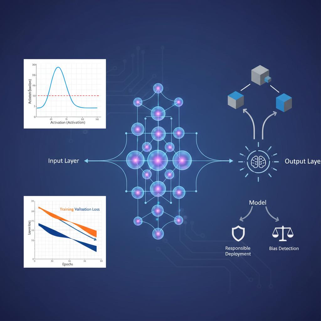
These individual neurons are organized into layers. A typical feedforward neural network consists of an input layer, which receives the raw data; one or more hidden layers, where the majority of the computation occurs; and an output layer, which produces the final prediction. The “depth” of a neural network refers to the number of hidden layers it contains.

Visual guide to activation dynamics

The activation function determines whether a neuron should be activated (“fire”) or not. Without these non-linear functions, a neural network, no matter how many layers it has, would behave like a simple linear model. Different activation functions have distinct properties that make them suitable for different tasks.

Activation Function	Characteristics	Common Use Case
Sigmoid	S-shaped curve that squashes outputs to a range between 0 and 1.	Output layer for binary classification problems.
Tanh (Hyperbolic Tangent)	Similar to sigmoid but squashes outputs to a range between -1 and 1.	Often used in hidden layers of older neural network architectures.
ReLU (Rectified Linear Unit)	Outputs the input if it is positive, otherwise outputs zero. It is computationally efficient.	The most common default choice for hidden layers in modern neural networks.
Leaky ReLU	A variant of ReLU that allows a small, non-zero gradient when the unit is not active.	Used to combat the “dying ReLU” problem where neurons can become inactive.

How learning happens: gradient descent and backpropagation

A neural network “learns” by adjusting its weights and biases to minimize the difference between its predictions and the actual ground truth. This process is framed as an optimization problem. First, we define a loss function (or cost function) that quantifies how “wrong” the model’s predictions are. Common examples include Mean Squared Error (MSE) for regression tasks and Cross-Entropy Loss for classification tasks.

The goal is to find the set of weights and biases that results in the lowest possible loss. This is achieved using an optimization algorithm called Gradient Descent. Imagine the loss function as a vast, hilly landscape where the altitude represents the loss. Our goal is to find the lowest point in this landscape. Gradient descent does this by taking small steps in the direction of the steepest descent—the negative gradient—of the loss function with respect to the model’s parameters. The size of these steps is controlled by a hyperparameter called the learning rate.

To perform gradient descent, we need to calculate the gradient of the loss function with respect to every weight and bias in the network. This is where backpropagation comes in. It is an efficient algorithm that computes these gradients by applying the chain rule of calculus, starting from the output layer and moving backward through the network. It calculates how much each parameter contributed to the overall error and determines how it should be adjusted to reduce that error.

Numerical stability, initialization, and scaling strategies

Training deep neural networks can be challenging due to numerical instability. A common issue is the vanishing or exploding gradient problem, where gradients become exponentially small or large as they are propagated backward through many layers, hindering learning. Looking ahead to 2026 and beyond, strategies for maintaining numerical stability remain a core focus of research.

• Weight Initialization: Proper initialization of weights is crucial. If weights are too large, gradients can explode; if they are too small, they can vanish. Techniques like Xavier/Glorot initialization and He initialization are designed to set initial weights to a suitable scale based on the number of input and output neurons.
• Feature Scaling: Input features should be scaled to a similar range, typically through standardization (zero mean, unit variance) or normalization (scaling to a [0, 1] range). This helps the gradient descent algorithm converge more smoothly and quickly.

Patterns in architecture: convolutional, recurrent, transformer style models and hybrids

While the basic feedforward network is a powerful tool, specialized architectures have been developed to handle specific types of data more effectively. These architectural patterns are the building blocks of most state-of-the-art AI systems.

• Convolutional Neural Networks (CNNs): Designed for grid-like data such as images. CNNs use special layers with learnable filters (or kernels) that slide across the input to detect features like edges, textures, and shapes. This allows them to learn spatial hierarchies efficiently, making them ideal for image classification and object detection.
• Recurrent Neural Networks (RNNs): Built for sequential data like time series or text. RNNs have loops, allowing information to persist in a “hidden state” that is passed from one step in the sequence to the next. This gives them a form of memory. Variants like LSTMs (Long Short-Term Memory) and GRUs (Gated Recurrent Units) were developed to better handle long-range dependencies.
• Transformer Models: A more recent architecture that has revolutionized natural language processing. Instead of processing sequences step-by-step like an RNN, Transformers use a mechanism called self-attention to weigh the importance of all words in the input sequence simultaneously. This parallel processing capability and its effectiveness at capturing long-range context have made it the dominant architecture for language tasks.
• Hybrid Models: It is also common to combine these patterns. For instance, a model for video analysis might use CNNs to extract features from each frame and an RNN or Transformer to model the temporal relationships between those features.

Training practices: regularization, normalization, and optimizer choices

Achieving high performance with neural networks requires more than just a good architecture; it demands disciplined training practices. A key challenge is overfitting, where a model learns the training data too well, including its noise, and fails to generalize to new, unseen data. Several techniques are used to combat this.

• Regularization: These are techniques that add a penalty to the loss function for model complexity. L1 and L2 regularization penalize large weight values. Dropout is another powerful method where a random fraction of neurons are temporarily “dropped” or ignored during each training step, forcing the network to learn more robust and redundant features.
• Normalization: Batch Normalization is a technique that normalizes the inputs to each layer for each mini-batch. This helps stabilize and accelerate the training process, often acting as a regularizer as well.
• Optimizers: While standard Gradient Descent is the conceptual basis, more advanced optimizers are used in practice. Optimizers like Adam, RMSprop, and Adagrad adapt the learning rate for each parameter individually, often leading to faster convergence than standard Stochastic Gradient Descent (SGD).

Measuring success: evaluation metrics and interpretability techniques

Evaluating a neural network’s performance requires choosing appropriate metrics. For classification tasks, accuracy is a common starting point, but it can be misleading on imbalanced datasets. It is often supplemented with:

• Precision: Of all the positive predictions, how many were actually correct?
• Recall (Sensitivity): Of all the actual positive cases, how many did the model correctly identify?
• F1-Score: The harmonic mean of precision and recall, providing a single score that balances both.

For regression tasks, Mean Absolute Error (MAE) and Mean Squared Error (MSE) are standard. Beyond quantitative metrics, understanding *why* a model makes a certain prediction is crucial for debugging, trust, and fairness. Interpretability techniques like SHAP (SHapley Additive exPlanations) and LIME (Local Interpretable Model-agnostic Explanations) help explain the output of complex models by highlighting which input features were most influential in a given prediction.

Safety and responsible design: bias, robustness, and governance

As neural networks become more integrated into critical applications, ensuring their safe and responsible deployment is paramount. Practitioners must address several key areas of AI Ethics and safety.

• Bias: Neural networks trained on biased data will learn and perpetuate those biases. It is critical to carefully audit datasets for demographic or historical biases and employ mitigation techniques during training and post-processing.
• Robustness: Models should be resilient to small, often imperceptible, perturbations in the input. Adversarial attacks are specifically crafted inputs designed to fool a model into making an incorrect prediction. Building robust models requires specialized training techniques and testing.
• Governance: Establishing clear governance frameworks for model development, deployment, and monitoring is essential. This includes documenting data sources, model architectures, and performance limitations to ensure transparency and accountability.

Reproducible experiments: synthetic cases and notebooks

Scientific rigor is as important in machine learning as in any other field. Reproducibility—the ability for others to achieve the same results with the same data and code—is a cornerstone of trustworthy research and development. To ensure your work with neural networks is reproducible, adopt practices such as:

• Version Control: Use tools like Git to track changes to code, model configurations, and documentation.
• Environment Management: Document all software dependencies and use tools like Docker or Conda to create consistent, shareable environments.
• Data and Model Versioning: Keep track of the exact dataset and model weights used for a given experiment.
• Experiment Tracking: Log hyperparameters, evaluation metrics, and other metadata for every training run. Using synthetic data for initial testing can also provide a controlled environment to validate model logic before moving to complex, real-world data.

From idea to model: building a simple network from scratch with pseudocode

To solidify these concepts, let’s outline the process of building and training a simple feedforward neural network with pseudocode. This example illustrates the core loop of training.

# 1. Define Network Architectureinput_size = 784hidden_size = 128output_size = 10learning_rate = 0.01# 2. Initialize Weights and BiasesW1 = initialize_weights(input_size, hidden_size)b1 = initialize_zeros(hidden_size)W2 = initialize_weights(hidden_size, output_size)b2 = initialize_zeros(output_size)# 3. Training Loopfor epoch in number_of_epochs:  for batch in training_data:    inputs, labels = batch    # --- Forward Pass ---    # Hidden layer    z1 = dot_product(inputs, W1) + b1    a1 = ReLU(z1)    # Output layer    z2 = dot_product(a1, W2) + b2    predictions = Softmax(z2) # Softmax for multi-class classification    # --- 4. Calculate Loss ---    loss = cross_entropy_loss(predictions, labels)    # --- 5. Backward Pass (Backpropagation) ---    # Calculate gradients for W2, b2, W1, b1    grad_z2 = predictions - labels    grad_W2 = dot_product(transpose(a1), grad_z2)    grad_b2 = sum(grad_z2)        grad_a1 = dot_product(grad_z2, transpose(W2))    grad_z1 = grad_a1 * ReLU_derivative(z1)    grad_W1 = dot_product(transpose(inputs), grad_z1)    grad_b1 = sum(grad_z1)    # --- 6. Update Weights and Biases ---    W1 = W1 - learning_rate * grad_W1    b1 = b1 - learning_rate * grad_b1    W2 = W2 - learning_rate * grad_W2    b2 = b2 - learning_rate * grad_b2

Further reading and curated resources

This whitepaper serves as a foundational introduction. To deepen your understanding of neural networks, we highly recommend the following resources:

• Deep Learning Textbook: An in-depth and comprehensive resource written by leading researchers in the field. It provides a strong theoretical foundation. You can find it at https://www.deeplearningbook.org.
• Visualizations and Blog Posts: Many online blogs provide excellent visual and intuitive explanations of complex topics. Exploring these can build a strong conceptual understanding to complement theoretical knowledge.

Summary and recommended next steps

We have journeyed from the basic building block of the artificial neuron to the complex architectures that power modern AI. We’ve covered how neural networks learn via gradient descent and backpropagation, explored key architectural patterns like CNNs and Transformers, and discussed the best practices for training, evaluation, and responsible deployment. The true power of these models lies not just in their predictive accuracy but in their ability to learn meaningful representations from vast amounts of data.

For practitioners and managers, the path forward involves continuous learning and hands-on application. We recommend the following next steps:

1. Implement a Simple Network: Move from pseudocode to actual code. Use a popular framework like TensorFlow or PyTorch to build and train a basic neural network on a classic dataset like MNIST.
2. Explore a Specific Architecture: Choose an architecture relevant to your domain—such as a CNN for image data or a Transformer for text—and complete a project using it.
3. Engage with the Community: Stay current with the latest research by following major conferences (e.g., NeurIPS, ICML) and engaging with the broader machine learning community.

By building a solid foundation in the principles of neural networks, you are well-equipped to innovate and lead in an era increasingly defined by artificial intelligence.