Neural Networks Explained: Concepts, Architecture and Training

Neural Networks Demystified: A Practitioner’s Guide to Architecture, Training, and Deployment

Table of Contents

• Executive summary — concise insights and practical implications
• A physical analogy: signals, weights, and adaptive pathways
• Core components: neurons, layers, and activation mechanisms
• How learning happens: loss, optimization, and backpropagation conceptually
• Architectural families and selection criteria
• Training at scale: data quality, regularization and validation
• Evaluation and interpretability: metrics and explanation techniques
• Deployment considerations: efficiency, monitoring and safety
• Responsible use: fairness, governance and security implications
• Case thought experiments: healthcare and finance scenarios
• Actionable checklist and curated resources for study
• Appendix: concise math primer and pseudocode examples

Executive summary — concise insights and practical implications

Neural Networks are computational models inspired by the structure and function of the human brain, forming the bedrock of modern artificial intelligence and deep learning. They excel at identifying complex patterns, making predictions, and classifying data in ways that traditional algorithms cannot. This whitepaper serves as a guide for intermediate to advanced practitioners, demystifying the core concepts of neural networks through intuitive analogies, exploring their architectural diversity, and providing a pragmatic framework for their training, deployment, and responsible governance. The key takeaway is that a neural network is not a black box but a system of weighted, interconnected components that learn to transform inputs into desired outputs by iteratively minimizing error. For technical leaders, understanding these mechanics is crucial for selecting appropriate architectures, diagnosing training issues, and implementing robust, ethical AI solutions that deliver tangible value while managing risk.

A physical analogy: signals, weights, and adaptive pathways

Imagine a complex network of water pipes, where each junction has a valve. Water (the input signal) enters from one end. At each junction (a neuron), the flow from multiple incoming pipes is combined. The valve at each incoming pipe (the weight) controls how much water it contributes to the mix. A pressure sensor at the junction (the activation function) measures the combined pressure. If the pressure exceeds a certain threshold, it opens a gate, allowing water to flow to the next set of pipes.

Initially, all the valves are set randomly. We want a specific amount of water to come out of specific pipes at the end of the network (the output). We measure the actual output, compare it to our desired output, and calculate the error. The process of “learning” is equivalent to sending a team of engineers backward through the pipe network. At each junction, they analyze the error and slightly adjust the valves (weights) that contributed most to the discrepancy. If a pipe let too much water through, its valve is tightened; if it let too little, it’s loosened. This process is repeated thousands or millions of times with different input flows, and with each iteration, the network of valves becomes better tuned to produce the desired output. This is the essence of how neural networks learn: by adjusting internal weights to map inputs to outputs.

Core components: neurons, layers, and activation mechanisms

At its core, a neural network is constructed from a few fundamental building blocks. Understanding these components is the first step toward mastering the design and implementation of these powerful models.

• Neurons (or Nodes): A neuron is the basic computational unit of a neural network. It receives one or more weighted inputs, applies an activation function to the sum of these inputs, and produces an output. Each neuron holds a bias, which is an additional, learnable parameter that allows it to shift the activation function output to the left or right, providing more modeling flexibility.
• Layers: Neurons are organized into layers. Every neural network has an input layer, which receives the initial data, and an output layer, which produces the final result. Between them are one or more hidden layers. It is the presence of these hidden layers that allows the network to learn complex, non-linear relationships in the data. Models with multiple hidden layers are referred to as “deep” neural networks, giving rise to the term deep learning.
• Weights and Connections: Each connection between neurons has an associated weight. This weight determines the strength and sign (excitatory or inhibitory) of the connection. The learning process of a neural network is fundamentally the process of finding the optimal set of weights that minimizes prediction error.

Activation functions explained intuitively

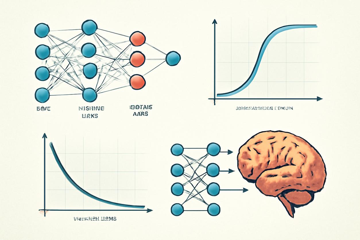
An activation function is a critical component that introduces non-linearity into the network, enabling it to learn more than just simple linear relationships. Without them, a multi-layer neural network would behave just like a single-layer linear model. Here are a few common types:

• Sigmoid: This function squashes any input value into a range between 0 and 1. It’s useful for output neurons in binary classification tasks, where the output can be interpreted as a probability.
• ReLU (Rectified Linear Unit): This is the most widely used activation function. It’s incredibly simple: it outputs the input directly if it’s positive, and outputs zero otherwise. This simplicity makes it computationally efficient and helps mitigate the vanishing gradient problem.
• Softmax: Used in the output layer of multi-class classification networks. It takes a vector of arbitrary real-valued scores and transforms them into a probability distribution, where each value is between 0 and 1, and all values sum to 1.

How learning happens: loss, optimization, and backpropagation conceptually

The “magic” of a neural network is its ability to learn from data. This learning process is an optimization problem that can be broken down into three conceptual steps: making a prediction, measuring the error, and updating the model to reduce that error.

1. Forward Propagation and Loss Calculation: Data is fed into the input layer and flows through the network, layer by layer, until it reaches the output layer. This is the forward pass. The network’s output is then compared to the true target value using a loss function (e.g., Mean Squared Error for regression or Cross-Entropy for classification). The loss function yields a single number that quantifies how “wrong” the network’s prediction was.
2. Backpropagation of Error: The core mechanism for learning is backpropagation. Conceptually, it is an algorithm for assigning blame. The loss value is propagated backward through the network. At each neuron, backpropagation calculates how much that neuron’s weights and bias contributed to the total error. This is done by calculating the gradient of the loss function with respect to each weight. For a deeper dive into the original concept, see the foundational paper on learning representations by back-propagating errors.
3. Optimization and Weight Update: An optimizer (e.g., Adam, SGD) uses the gradients calculated during backpropagation to update the network’s weights. It takes a small step in the direction opposite to the gradient, effectively nudging the weights in a direction that minimizes the loss. This entire cycle—forward pass, loss calculation, backpropagation, and weight update—is called an epoch, and it is repeated until the model’s performance on a validation dataset stops improving.

Common optimization behaviours and troubleshooting

During training, practitioners often encounter specific behaviors that require diagnosis:

• Learning Rate Too High: The loss may fluctuate wildly or even increase. The optimizer is “overshooting” the minimum of the loss landscape. Solution: Decrease the learning rate.
• Learning Rate Too Low: The loss decreases very slowly, and training takes an excessively long time. The optimizer is taking tiny, inefficient steps. Solution: Increase the learning rate or use an adaptive optimizer like Adam.
• Plateauing Loss: The loss decreases and then flattens out. This could mean the model has converged, or it’s stuck in a local minimum. Solution: Try a different optimizer, adjust the learning rate, or increase model complexity.

Architectural families and selection criteria

Not all neural networks are structured the same. Different architectures are designed to excel at specific types of tasks and data. Choosing the right architecture is a critical decision based on the problem at hand.

• Feedforward Neural Networks (FNNs): The simplest type, where information moves in only one direction—forward. They are excellent for structured data tasks like tabular classification or regression.
• Convolutional Neural Networks (CNNs): The gold standard for image and video data. CNNs use special layers with “filters” that scan across an image to detect patterns like edges, textures, and shapes, preserving spatial hierarchies.
• Recurrent Neural Networks (RNNs): Designed for sequential data like time series or natural language. RNNs have loops, allowing information to persist. Variants like LSTM (Long Short-Term Memory) and GRU (Gated Recurrent Unit) solve issues with long-term dependencies.
• Transformers: A more recent architecture that has revolutionized natural language processing (NLP). Instead of sequential processing, it uses an attention mechanism to weigh the importance of different words in a sequence simultaneously, enabling a deeper understanding of context.

Convolutional patterns, sequence models and attention mechanisms

The innovation within these families lies in their specialized layers. CNNs use convolutional layers to learn spatial features. RNNs use recurrent connections to maintain a “memory” of past inputs. Transformers rely entirely on self-attention, a mechanism that allows the model to look at other parts of the input sequence for clues that can help lead to a better encoding for a specific word or token. This is what allows models like GPT to understand nuanced language and context so effectively.

Training at scale: data quality, regularization and validation

Training large-scale neural networks effectively requires more than just a powerful algorithm; it demands a disciplined approach to data management, model validation, and preventing common pitfalls.

• Data Quality and Quantity: The performance of any neural network is capped by the quality of its training data. A large, diverse, and well-labeled dataset is paramount. Data preprocessing steps like normalization (scaling data to a standard range) and augmentation (creating modified copies of data to expand the dataset) are standard practice.
• Regularization: These are techniques used to prevent overfitting, where a model learns the training data too well, including its noise, and fails to generalize to new, unseen data. Common methods include Dropout (randomly “turning off” a fraction of neurons during training) and L1/L2 regularization (adding a penalty to the loss function based on the magnitude of the model weights).
• Validation Strategy: It’s crucial to split data into three sets: a training set to fit the model, a validation set to tune hyperparameters (like learning rate or model architecture), and a test set to provide an unbiased evaluation of the final model’s performance. Cross-validation is a robust technique for getting a more reliable estimate of model performance.

Avoiding overfitting and mitigating bias

Overfitting is a constant battle. Besides regularization, other strategies include early stopping, where training is halted once performance on the validation set starts to degrade. Mitigating bias is equally critical. If the training data is not representative of the real-world population, the neural network will learn and amplify these biases. This requires careful data auditing, and potentially using techniques like re-sampling or algorithmic fairness constraints during training.

Evaluation and interpretability: metrics and explanation techniques

Once a neural network is trained, its performance must be rigorously evaluated. The choice of metrics depends on the task. For classification, metrics like accuracy, precision, recall, and the F1-score are common. For regression, Mean Absolute Error (MAE) or Root Mean Squared Error (RMSE) are used.

However, performance metrics only tell part of the story. Interpretability—understanding *why* a model made a particular decision—is increasingly important, especially in high-stakes domains. Techniques like SHAP (SHapley Additive exPlanations) and LIME (Local Interpretable Model-agnostic Explanations) help explain individual predictions by highlighting which input features were most influential. This is a rapidly evolving field, and staying current with the literature, such as this interpretability survey, is vital for practitioners.

Deployment considerations: efficiency, monitoring and safety

Moving a trained neural network from a research environment to a production system introduces a new set of challenges.

• Efficiency: Large models can be computationally expensive. Techniques like quantization (reducing the precision of model weights) and pruning (removing unimportant connections) can significantly reduce model size and inference latency without a major drop in accuracy.
• Monitoring: Post-deployment, models must be continuously monitored for performance degradation and model drift, which occurs when the statistical properties of the production data change over time. Monitoring systems should track key metrics and trigger alerts for retraining when necessary.
• Safety and Robustness: In production, models can be exposed to adversarial attacks—subtly modified inputs designed to cause incorrect predictions. Future-proofing your MLOps strategies for 2025 and beyond will require building robust defenses and conducting rigorous testing against such vulnerabilities.

Responsible use: fairness, governance and security implications

The power of neural networks comes with significant responsibility. Practitioners and organizations must address the ethical dimensions of their application.

• Fairness and Bias: As mentioned, models can perpetuate societal biases present in data. Auditing for fairness across different demographic groups and implementing mitigation techniques is a non-negotiable step.
• Governance and Transparency: Organizations need clear governance frameworks for AI development. This includes documenting data sources, model architectures, and training procedures to ensure reproducibility and accountability. Emerging governance frameworks expected post-2025 will likely mandate even stricter transparency and documentation standards.
• Security: Beyond adversarial attacks, neural networks can be vulnerable to data privacy issues, such as model inversion attacks that can reconstruct sensitive training data from model outputs. Techniques like federated learning and differential privacy offer ways to train models without centralizing or exposing raw user data.

Case thought experiments: healthcare and finance scenarios

To ground these concepts, consider two scenarios:

• Healthcare: A CNN is trained on millions of retinal scans to detect diabetic retinopathy. The model achieves high accuracy but is a black box. Interpretability techniques (like SHAP) could highlight the specific pixels or regions of the eye that led to a positive diagnosis, giving clinicians confidence and a tool for double-checking the AI’s reasoning. The deployment plan must include monitoring for drift as new imaging equipment is introduced in hospitals.
• Finance: A transformer-based model is used for credit scoring by analyzing an applicant’s financial history. A key responsibility challenge is ensuring the model is not biased against protected groups. This requires rigorous fairness audits and a governance model that allows for clear explanations of credit denials, as required by regulations.

Actionable checklist and curated resources for study

For practitioners looking to develop and deploy neural networks effectively:

• Problem Framing: Is a neural network the right tool for this problem? Have you established clear success metrics?
• Data Foundation: Is your data clean, representative, and sufficient? Do you have a strategy for mitigating bias?
• Architecture Selection: Have you chosen an architecture (e.g., CNN, Transformer) that matches your data type and problem?
• Training and Validation: Do you have a robust validation strategy? Are you using regularization and monitoring for overfitting?
• Deployment and MLOps: How will you optimize the model for inference? How will you monitor for drift and retrain?
• Responsibility and Governance: Have you assessed fairness, security, and interpretability needs?

For continued learning, the following resources are invaluable:

• A comprehensive deep learning overview for a broad perspective.
• The seminal “Deep Learning” book by Goodfellow, Bengio, and Courville, available at deeplearningbook.org.

Appendix: concise math primer and pseudocode examples

While this guide is conceptually focused, a brief look at the underlying mechanics is helpful.

Core Calculation (Neuron):

output = activation_function( (sum(weights * inputs)) + bias )

Pseudocode for a Training Step:

for epoch in number_of_epochs: for data_batch in training_data: # Forward pass predictions = model.forward(data_batch.inputs) # Calculate error loss = loss_function(predictions, data_batch.labels) # Backward pass gradients = loss.backward() # Update weights optimizer.step(gradients, learning_rate)

This pseudocode encapsulates the iterative learning loop that is fundamental to all supervised training of neural networks. By repeatedly adjusting its internal weights based on the calculated error, the network gradually improves its ability to map inputs to correct outputs.