A Practical Guide to Neural Networks: From Theory to Deployment
Table of Contents
- Introducing Neural Networks: Intuition and History
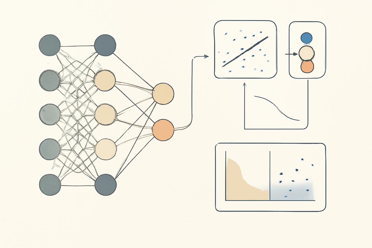
- Anatomy of a Network: Neurons, Layers and Activations
- Architectures and When to Use Them
- Training Fundamentals: Loss, Optimization and Regularization
- Practical Workflow: Datasets to Deployment
- Responsible Use: Explainability, Fairness and Robustness
- Hands-on Resources: Minimal Notebooks, Sample Code and Further Reading
- Conclusion: Next Steps for Experimentation
Introducing Neural Networks: Intuition and History
At its core, a Neural Network is a computational model inspired by the human brain. It’s designed to recognize patterns in data by processing information through a series of interconnected nodes, much like our own biological neurons. While the foundational concepts date back to the mid-20th century, the recent explosion in computational power and data availability has catapulted neural networks to the forefront of artificial intelligence, powering everything from image recognition and natural language processing to self-driving cars.
Think of a neural network as a highly adaptable function approximator. You provide it with inputs (like an image) and the desired outputs (like the label “cat”), and during a process called training, it learns the intricate mathematical function that maps one to the other. This ability to learn complex, non-linear relationships directly from data is what makes neural networks so powerful and versatile.
Anatomy of a Network: Neurons, Layers and Activations
To truly understand neural networks, we must first dissect their fundamental components. These models are built from simple units that, when combined, exhibit complex emergent behavior.
The basic building blocks include:
- Neurons (or Nodes): A neuron is the primary computational unit. It receives one or more inputs, performs a simple calculation, and produces an output. Each input is multiplied by a weight, which signifies the input’s importance. The weighted inputs are summed, a bias term is added, and the result is passed through an activation function.
- Layers: Neurons are organized into layers. A typical neural network has at least three types of layers:
- Input Layer: This is the entry point for your data. The number of neurons in this layer corresponds to the number of features in your dataset (e.g., for a 28×28 pixel image, you’d have 784 input neurons).
- Hidden Layers: These are the layers between the input and output. It’s where the magic happens. A network can have one or many hidden layers, and the term “deep learning” refers to neural networks with multiple hidden layers. They are responsible for learning progressively more complex features from the data.
- Output Layer: This final layer produces the network’s prediction. The number of neurons and the activation function used here depend entirely on the task (e.g., one neuron for regression, or multiple neurons with a softmax activation for multi-class classification).
Activation Functions Explained
An activation function is a crucial component of a neuron. It introduces non-linearity into the network, allowing it to learn far more complex patterns than a simple linear model could. Without them, a deep stack of layers would be mathematically equivalent to a single, much simpler layer. Common activation functions include:
- Sigmoid: Squashes values to a range between 0 and 1. It’s often used in the output layer for binary classification tasks but can suffer from the “vanishing gradient” problem in deep networks.
- Tanh (Hyperbolic Tangent): Similar to sigmoid but squashes values to a range between -1 and 1. It’s zero-centered, which can help with optimization.
- ReLU (Rectified Linear Unit): This is the most popular activation function for hidden layers. It outputs the input directly if it is positive, and zero otherwise. It’s computationally efficient and helps mitigate the vanishing gradient problem.
- Leaky ReLU: A variation of ReLU that allows a small, non-zero gradient when the unit is not active, preventing “dying neurons.”
- Softmax: Exclusively used in the output layer for multi-class classification. It converts a vector of numbers into a probability distribution, where each value represents the probability of the input belonging to a particular class.
Architectures and When to Use Them
Not all neural networks are created equal. Different problems require different architectures designed to best capture the underlying patterns in the data.
Feedforward and Convolutional Networks
Feedforward Neural Networks (FNNs), also known as Multi-Layer Perceptrons (MLPs), are the simplest type. Information flows in only one direction—from the input layer, through the hidden layers, to the output layer. There are no cycles or loops. They are excellent for structured data tasks, such as tabular data classification or regression.
Convolutional Neural Networks (CNNs) are a specialized type of neural network designed for processing grid-like data, most notably images. They use a special layer called a convolutional layer, which applies filters (kernels) across the input to learn spatial hierarchies of features. For example, a first layer might learn to detect edges, a second might combine edges to detect shapes, and a third might combine shapes to detect objects. This makes them incredibly effective for image classification, object detection, and image segmentation.
Recurrent and Transformer-Style Architectures
Recurrent Neural Networks (RNNs) are designed to work with sequential data, like time series or text. They have loops that allow information to persist, giving them a form of “memory.” This enables them to understand context based on previous inputs in the sequence. LSTMs (Long Short-Term Memory) and GRUs (Gated Recurrent Units) are advanced types of RNNs that solve some of the original architecture’s limitations with long-term dependencies.
Transformer architectures have largely superseded RNNs for many natural language processing (NLP) tasks. Instead of processing data sequentially, they use a mechanism called “self-attention” to weigh the importance of different words in the input data simultaneously. This parallel processing capability and superior handling of long-range dependencies have made them the foundation for state-of-the-art models like BERT and GPT.
Training Fundamentals: Loss, Optimization and Regularization
Training is the process of teaching a neural network to perform a task. It’s an iterative process that involves showing the model data, measuring its error, and adjusting its internal parameters (weights and biases) to reduce that error.
- Loss Function (or Cost Function): This function measures how wrong the model’s prediction is compared to the true label. The choice of loss function depends on the task (e.g., Mean Squared Error for regression, Cross-Entropy for classification). The goal of training is to minimize this value.
- Optimizer: This is the algorithm that implements the backpropagation process, adjusting the network’s weights to minimize the loss. It calculates the gradient of the loss function with respect to each weight and nudges the weight in the opposite direction.
- Regularization: These are techniques used to prevent the model from “memorizing” the training data, a phenomenon known as overfitting. A well-regularized model generalizes better to new, unseen data.
Common Optimization Algorithms
Choosing the right optimizer can significantly impact training speed and model performance. While Gradient Descent is the foundational concept, several more advanced algorithms are used in practice:
- Stochastic Gradient Descent (SGD) with Momentum: An enhancement to standard SGD that helps accelerate convergence, especially in high-curvature areas of the loss landscape.
- RMSprop: An adaptive learning rate method that divides the learning rate by an exponentially decaying average of squared gradients.
- Adam (Adaptive Moment Estimation): This is arguably the most popular and often default optimizer. It combines the ideas of momentum and RMSprop, maintaining both an adaptive learning rate for each parameter and a momentum term.
Overfitting and Mitigation Strategies
Overfitting occurs when a model learns the training data too well, including its noise and idiosyncrasies, leading to poor performance on unseen data. Key mitigation strategies for any 2025 deep learning project include:
- L1 and L2 Regularization: These techniques add a penalty to the loss function based on the magnitude of the model’s weights. This encourages the model to use smaller, more uniform weights, making it less complex.
- Dropout: During training, this technique randomly sets a fraction of neuron activations to zero at each update. This forces the network to learn more robust features and prevents it from becoming too reliant on any single neuron.
- Early Stopping: Monitor the model’s performance on a separate validation dataset during training. If the validation performance stops improving (or starts to degrade) for a certain number of epochs, training is stopped to prevent further overfitting.
- Data Augmentation: Artificially increase the size and diversity of your training dataset by creating modified copies of existing data (e.g., rotating, cropping, or flipping images).
Practical Workflow: Datasets to Deployment
Building effective neural networks involves a systematic workflow from data handling to production monitoring.
Data Preparation and Augmentation
Garbage in, garbage out. The quality of your data is paramount. This stage involves:
- Data Cleaning: Handling missing values and correcting errors.
- Feature Scaling: Normalizing or standardizing numerical features (e.g., scaling to a range of [0, 1] or to a mean of 0 and standard deviation of 1). This helps optimization algorithms converge faster.
- Encoding: Converting categorical features into a numerical format that the neural network can understand (e.g., one-hot encoding).
As mentioned earlier, data augmentation is a powerful technique to improve model robustness, especially when training data is limited.
Model Evaluation and Monitoring
After training, you must evaluate your model’s performance on a held-out test set. Key metrics depend on the task:
- Classification: Accuracy, Precision, Recall, F1-Score, and the Confusion Matrix are standard.
- Regression: Mean Absolute Error (MAE), Mean Squared Error (MSE), and R-squared are commonly used.
Once deployed, a model’s work is not done. Continuous monitoring is essential to detect model drift—a degradation in performance over time as the real-world data distribution changes. This requires a robust MLOps pipeline to track performance and trigger retraining when necessary.
Responsible Use: Explainability, Fairness and Robustness
As neural networks become more integrated into critical systems, their responsible use is a major concern. It’s not enough for a model to be accurate; it must also be trustworthy.
- Explainability (XAI): Many neural networks are “black boxes.” Explainability techniques like SHAP and LIME help us understand *why* a model made a particular prediction, which is crucial for debugging, validation, and building user trust.
- Fairness: Models trained on biased data will produce biased outcomes. It’s essential to audit datasets and model predictions for demographic biases and apply fairness mitigation techniques to ensure equitable outcomes.
- Robustness: This refers to a model’s ability to maintain performance under unexpected or adversarial conditions. Testing against adversarial attacks (subtly perturbed inputs designed to fool the model) is an important step in building secure AI systems.
Hands-on Resources: Minimal Notebooks, Sample Code and Further Reading
The best way to learn is by doing. The theoretical foundation is vital, but practical application solidifies understanding. Here are some invaluable resources for intermediate practitioners:
- Deep Learning Book: Written by Goodfellow, Bengio, and Courville, this is the definitive theoretical textbook for those wanting to dive deep into the mathematics and concepts behind neural networks.
- Minimal Notebooks: A great learning strategy is to build neural networks from scratch using libraries like NumPy before moving to frameworks like TensorFlow or PyTorch. This reveals the inner workings of processes like backpropagation.
- Papers With Code: This resource is indispensable for staying current. It links state-of-the-art research papers with their corresponding code implementations, allowing you to explore and run the latest models.
- arXiv Machine Learning: For the absolute cutting edge, the cs.LG (Machine Learning) section of arXiv is where most new research papers are published first. It’s a firehose of information but essential for seeing what’s on the horizon.
Conclusion: Next Steps for Experimentation
We’ve journeyed from the basic neuron to the complexities of training, deployment, and responsible AI. Neural networks are a vast and rapidly evolving field, but the core principles provide a solid foundation for exploration. Your next step is to apply these concepts. Pick a clean dataset, choose a simple architecture like an FNN, and walk through the entire workflow: data preparation, model training, evaluation, and iteration. By bridging the gap between theory and practice, you can begin to effectively harness the transformative power of neural networks to solve real-world problems.


