Inside Neural Networks: Principles, Architectures and Practical Uses

Executive Summary

Neural networks represent a cornerstone of modern artificial intelligence (AI) and machine learning, driving innovations from autonomous systems to personalized medicine. This whitepaper serves as a comprehensive guide for practitioners, data scientists, and technical managers. It bridges the gap between the theoretical underpinnings of neural networks and the practical realities of their implementation. We explore foundational concepts, mathematical principles, common architectures, and end-to-end workflows from training to deployment. Furthermore, this document emphasizes the critical importance of interpretability, ethical governance, and responsible AI practices. By providing reproducible pseudocode, domain-specific case studies, and a look into future research, this paper equips readers with the knowledge to design, build, and manage robust and effective neural network solutions.

Why Neural Networks Matter Today

The resurgence and current dominance of neural networks, particularly deep learning models, are fueled by three primary factors: the availability of massive datasets, significant advancements in parallel computing hardware (like GPUs and TPUs), and the development of more sophisticated algorithms and software frameworks (e.g., TensorFlow, PyTorch). Unlike traditional machine learning algorithms that often require manual feature engineering, neural networks can learn hierarchical representations of features directly from raw data. This capability makes them exceptionally powerful for tackling complex, high-dimensional problems such as image recognition, natural language processing, and time-series analysis, which were previously intractable. Their ability to model non-linear relationships with high accuracy has positioned neural networks as the engine behind many of today’s technological breakthroughs.

Foundational Concepts and Intuitions

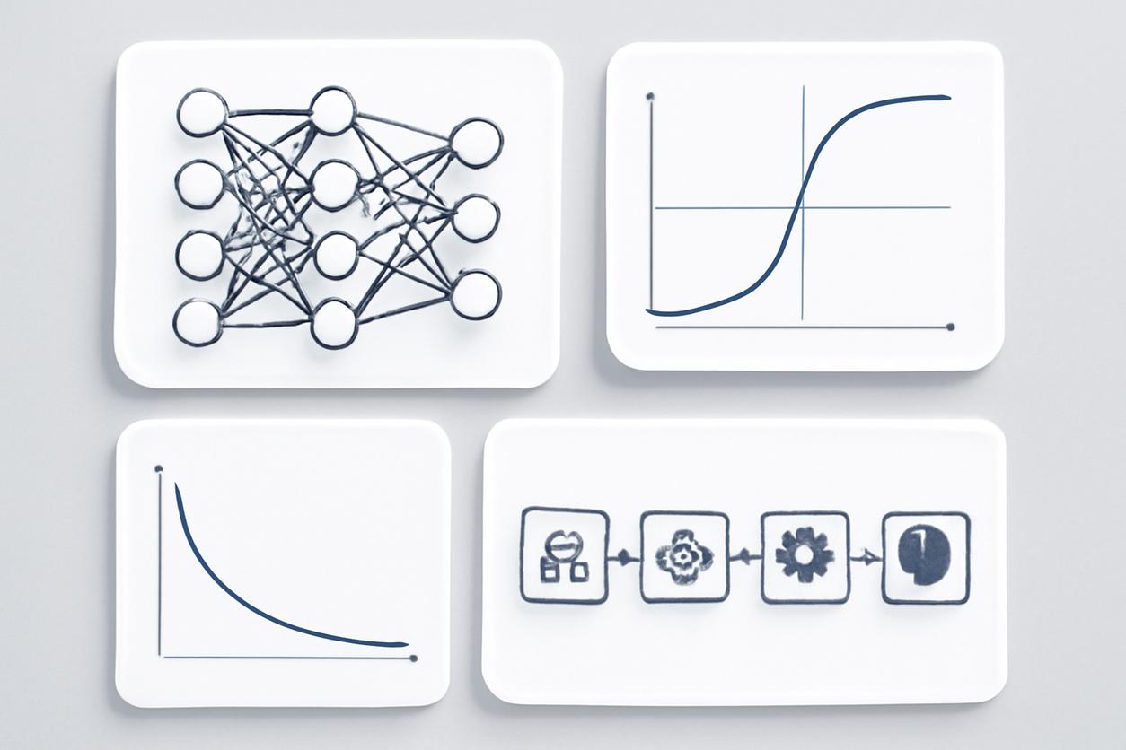
At its core, an artificial neural network is a computational model inspired by the structure and function of the human brain. It is comprised of interconnected nodes, or neurons, organized in layers. The fundamental idea is to process information in a way that mimics biological neural systems. For a detailed overview, see the Neural Networks overview on Wikipedia.

The Artificial Neuron

The basic unit of a neural network is the neuron, also known as a perceptron in simpler models. A neuron receives one or more inputs, performs a weighted sum of these inputs, adds a bias, and then passes the result through an activation function. This function introduces non-linearity, enabling the network to learn complex patterns.

• Inputs (x): The data fed into the neuron.
• Weights (w): Parameters that the network learns. They determine the strength of the connection between neurons.
• Bias (b): A parameter that allows shifting the activation function, increasing model flexibility.
• Activation Function (f): A function like Sigmoid, ReLU, or Tanh that transforms the neuron’s output.

Layers and Architecture

Neurons are organized into layers:

• Input Layer: Receives the initial raw data. The number of neurons in this layer corresponds to the number of features in the dataset.
• Hidden Layers: Sit between the input and output layers. This is where most of the computation and feature extraction occurs. A neural network with one or more hidden layers is considered a “deep” neural network.
• Output Layer: Produces the final result, such as a classification (e.g., ‘cat’ or ‘dog’) or a regression value (e.g., a stock price).

Information flows from the input layer, through the hidden layers, to the output layer in a process known as forward propagation. The network’s ability to learn comes from adjusting the weights and biases to minimize the difference between its predictions and the actual ground truth, a process called training.

Mathematical Building Blocks

Understanding the core mathematical concepts is essential for any practitioner working with neural networks. While modern frameworks abstract away many of these details, a grasp of the underlying principles is crucial for debugging, optimization, and advanced model design.

Key Components

• Linear Algebra: Operations like matrix multiplication and vector addition are fundamental. Data, weights, and biases are all represented as tensors (multi-dimensional arrays), and forward propagation is essentially a series of tensor operations.
• Calculus: The concept of the derivative is central to training. The gradient, a multi-variable generalization of the derivative, indicates the direction of steepest ascent for a function. During training, we use gradients to descend the loss function and find the optimal weights.
• Probability and Statistics: Loss functions, activation functions (like Softmax), and model initialization techniques are rooted in probabilistic principles. Understanding distributions and statistical measures is key to evaluating model performance.

The training process relies on an algorithm called backpropagation, which is a practical application of the chain rule from calculus. It efficiently calculates the gradient of the loss function with respect to every weight and bias in the network, enabling the model to learn from its errors.

Common Architectures and Selection Guidance

Different problems require different types of neural network architectures. Selecting the right one is critical for success.

Architecture Overview Table

Architecture	Primary Use Case	Key Characteristics
Feedforward Neural Networks (FNNs)	Tabular data, regression, basic classification	Information flows in one direction; no loops. The simplest form of neural networks.
Convolutional Neural Networks (CNNs)	Image and video analysis, computer vision	Uses convolutional layers to detect spatial hierarchies of features (e.g., edges, shapes, objects).
Recurrent Neural Networks (RNNs)	Sequential data: time series, natural language	Contains loops, allowing information to persist. Good for modeling sequences and dependencies.
Long Short-Term Memory (LSTM) / Gated Recurrent Unit (GRU)	Advanced sequential data tasks	Variants of RNNs designed to overcome the vanishing gradient problem and learn long-term dependencies.
Transformers	Natural Language Processing (NLP), vision	Relies on self-attention mechanisms to weigh the importance of different parts of the input data. State-of-the-art for many NLP tasks.

Selection Guidance

When choosing an architecture, consider the nature of your data and the problem you are trying to solve. For image data, a CNN is almost always the starting point. For text or time-series data, LSTMs or Transformers are appropriate. For structured, tabular data, a simple FNN or a gradient boosting model may be sufficient. Stanford’s CS231n course notes provide excellent visual and practical explanations of these architectures, particularly for computer vision.

Training Workflows and Optimization Strategies

Training a neural network is an iterative process of optimizing its parameters to minimize a loss function.

The Training Loop

A standard training workflow involves these steps, repeated over many epochs (passes through the entire dataset):

1. Data Preparation: Split data into training, validation, and test sets. Preprocess by normalizing, standardizing, or augmenting the data.
2. Forward Pass: Pass a batch of training data through the network to generate predictions.
3. Loss Calculation: Compare the predictions to the true labels using a loss function (e.g., Mean Squared Error for regression, Cross-Entropy for classification).
4. Backward Pass (Backpropagation): Calculate the gradients of the loss with respect to the network’s parameters.
5. Parameter Update: Adjust the parameters using an optimizer to reduce the loss.

Optimization Strategies for 2025 and Beyond

Effective optimization is key to achieving high performance. Modern strategies focus on efficiency and stability:

• Advanced Optimizers: While Stochastic Gradient Descent (SGD) is the classic, adaptive optimizers like Adam, AdamW, and RAdam are standard. Future research in 2025 will likely focus on optimizers that require even less hyperparameter tuning and perform well across diverse architectures.
• Learning Rate Scheduling: Instead of a fixed learning rate, dynamically adjusting it during training often improves performance. Techniques like cosine annealing, cyclical learning rates, and one-cycle policies will continue to be refined.
• Batch Size Selection: The choice of batch size impacts convergence speed and generalization. Techniques for adaptive batch sizing and navigating the trade-offs between small and large batches will be a key strategic consideration.

Regularization, Evaluation, and Debugging Methods

A trained model is only useful if it generalizes well to unseen data. This requires robust regularization, evaluation, and debugging.

Regularization to Prevent Overfitting

Overfitting occurs when a model learns the training data too well, including its noise, and fails to generalize. Regularization techniques help prevent this:

• L1 and L2 Regularization: Adds a penalty to the loss function based on the magnitude of the model’s weights.
• Dropout: During training, randomly sets a fraction of neuron activations to zero at each update step, forcing the network to learn more robust features.
• Data Augmentation: Artificially expands the training dataset by creating modified copies of existing data (e.g., rotating or cropping images).
• Early Stopping: Monitors the model’s performance on a validation set and stops training when performance ceases to improve.

Evaluation Metrics and Debugging

Choose metrics that align with your business goal. For classification, this could be accuracy, precision, recall, F1-score, or AUC-ROC. For regression, use Mean Absolute Error (MAE) or Root Mean Squared Error (RMSE). When a neural network underperforms, common debugging steps include: visualizing the loss curve, checking for correct data preprocessing, starting with a simpler model, and verifying the implementation of backpropagation.

Interpretability and Model Introspection

As neural networks are deployed in high-stakes domains, understanding *why* a model makes a certain prediction is crucial. This is the field of eXplainable AI (XAI).

Techniques for Interpretability

• Feature Importance: Methods like SHAP (SHapley Additive exPlanations) and LIME (Local Interpretable Model-agnostic Explanations) assign an importance value to each input feature for a given prediction.
• Saliency Maps: For CNNs, these are heatmaps that highlight which pixels in an input image were most influential in the model’s decision.
• Activation Maximization: A technique to visualize what a particular neuron or layer has learned to detect by generating an input that maximally activates it.

Building interpretable models fosters trust, aids in debugging, ensures fairness, and is often a regulatory requirement.

Deployment Pipeline and Scalability Considerations

Moving a neural network from a research environment to a production system requires a well-defined MLOps (Machine Learning Operations) pipeline.

Key Pipeline Stages

1. Model Packaging: Saving the trained model architecture and weights in a serialized format (e.g., ONNX, SavedModel).
2. Serving Infrastructure: Deploying the model via a REST API endpoint, often within a containerized environment like Docker.
3. Performance Optimization: Using techniques like quantization (reducing numerical precision) and model pruning to decrease latency and computational cost.
4. Monitoring and Maintenance: Continuously monitoring model performance, data drift, and concept drift to know when retraining is necessary.

Scalability requires designing systems that can handle varying loads, often leveraging cloud services for elastic compute and managed model serving.

Domain Case Studies: Healthcare, Finance, and Automation

The impact of neural networks is evident across numerous industries.

• Healthcare: CNNs are used for medical image analysis, detecting diseases like cancer from X-rays and MRIs with superhuman accuracy. RNNs and Transformers model patient data over time to predict disease progression.
• Finance: Neural networks are applied in algorithmic trading, credit scoring, and fraud detection. LSTMs are particularly effective for time-series forecasting of market trends.
• Automation: In robotics and autonomous vehicles, neural networks process sensor data (from cameras, LiDAR) for object detection, path planning, and decision-making.

Responsible AI: Risks, Governance, and Compliance

Deploying AI, especially complex neural networks, carries significant responsibilities. A framework for Responsible AI is essential.

Core Pillars

• Fairness and Bias: Neural networks trained on biased data will perpetuate and even amplify those biases. Auditing datasets and models for fairness across demographic groups is critical.
• Privacy: Techniques like federated learning and differential privacy allow for training models without centralizing sensitive user data.
• Accountability and Transparency: Maintaining clear documentation, version control for models and data, and using interpretable models are key to establishing accountability.
• Security: Protecting models from adversarial attacks, where malicious inputs are designed to fool the model, is a growing area of concern.

Organizations should align their AI governance with established frameworks and guidelines, such as those provided by the NIST Artificial Intelligence Resources, to ensure compliance and build trust.

Hands-on Reproducible Example in Pseudocode

This pseudocode illustrates the fundamental training loop of a simple feedforward neural network.

function train_neural_network(training_data, labels, epochs, learning_rate):    // 1. Initialize network with random weights and biases    // Structure: input layer, one hidden layer, output layer    network = initialize_network(input_size, hidden_size, output_size)    // 2. Loop for a number of epochs    for epoch in 1 to epochs:        total_loss = 0        // Iterate over each data point (in practice, this is done in batches)        for data_point, true_label in zip(training_data, labels):            // 3. Forward Propagation: Pass data through the network            prediction = forward_pass(network, data_point)            // 4. Calculate Loss: Measure the error            loss = calculate_cross_entropy_loss(prediction, true_label)            total_loss += loss            // 5. Backward Propagation: Calculate gradients            gradients = backpropagate(network, loss)            // 6. Update Weights and Biases            network = update_parameters(network, gradients, learning_rate)        print("Epoch: ", epoch, " Average Loss: ", total_loss / len(training_data))    return network// Helper functions (definitions omitted for brevity)function initialize_network(input_size, hidden_size, output_size): ...function forward_pass(network, input_data): ...function calculate_cross_entropy_loss(prediction, true_label): ...function backpropagate(network, loss): ...function update_parameters(network, gradients, learning_rate): ...

Future Research Trajectories and Open Problems

The field of neural networks is evolving rapidly. Key research areas for 2025 and beyond include:

• Efficient Models: Developing architectures that require less data and computational power to train, making deep learning more accessible and sustainable (e.g., TinyML, hardware-aware model design).
• Neuro-symbolic AI: Combining neural networks’ pattern recognition capabilities with symbolic reasoning to achieve more robust and generalizable intelligence.
• Self-supervised Learning: Training models on vast amounts of unlabeled data, reducing the dependency on expensive, manually labeled datasets.
• Causality: Moving beyond correlation to understand and model causal relationships, enabling models to reason about interventions and counterfactuals.

Appendix: Concise Math Refresher

• Dot Product: The sum of the products of corresponding entries of two sequences of numbers. Central to calculating a neuron’s pre-activation value. z = w ⋅ x + b
• Matrix Multiplication: The core operation for processing a layer of neurons or a batch of data simultaneously.
• Chain Rule: A formula to compute the derivative of a composite function. Backpropagation is a recursive application of the chain rule. d/dx[f(g(x))] = f'(g(x)) * g'(x)
• Gradient Descent: An iterative optimization algorithm for finding a local minimum of a differentiable function. The weight update rule is: w_new = w_old – learning_rate * ∇Loss(w_old)

References and Further Reading

For those seeking to deepen their understanding of neural networks, the following resources are invaluable:

• Deep Learning by Ian Goodfellow, Yoshua Bengio, and Aaron Courville: Often considered the foundational textbook on the subject. Available online at www.deeplearningbook.org.
• Stanford CS231n: Convolutional Neural Networks for Visual Recognition: Comprehensive course notes, lectures, and assignments that provide practical insights into building neural networks. Available at cs231n.github.io.
• NIST Artificial Intelligence Resource Center: A collection of standards, guidelines, and research for developing trustworthy and responsible AI systems. Explore their resources at www.nist.gov/artificial-intelligence.