Neural Networks Explained: From Intuition to Application

Neural Networks: A Data Scientist’s Deep Dive from Foundations to Deployment

Table of Contents

• Introduction: Why Neural Networks Matter
• Foundations: Neurons, Layers and Activation Functions
• How Learning Happens: Loss, Backpropagation and Optimization
• Architectures Demystified: Feedforward, Convolutional, Recurrent and Transformer Models
• Training Strategies: Data, Regularization and Hyperparameter Tuning
• Interpreting Models: Visualization and Explainability Techniques
• Practical Walkthrough: Designing a Simple Classifier Step by Step
• Evaluation and Validation: Metrics and Robust Testing
• Deployment Notes: From Prototype to Scalable Serving
• Ethics and Safety: Responsible AI Practices for Models
• Troubleshooting: Common Failure Modes and Remedies
• Resources for Continued Learning
• Summary and Next Steps

Introduction: Why Neural Networks Matter

In the vast landscape of artificial intelligence, few concepts have been as transformative as neural networks. These powerful computational models, inspired by the intricate architecture of the human brain, are the engine behind today’s most significant AI breakthroughs—from self-driving cars that navigate complex city streets to natural language models that can write poetry or translate languages in real time. For data scientists, machine learning engineers, and technical leaders, a deep understanding of neural networks is no longer optional; it is fundamental.

This whitepaper serves as a comprehensive guide, designed to demystify the core concepts of neural networks. We will move from the foundational building blocks of neurons and layers to the sophisticated dynamics of training and deployment. By combining intuitive analogies with practical considerations, this article will equip you with the knowledge to not only understand how neural networks work but also how to build, evaluate, and deploy them responsibly.

Foundations: Neurons, Layers and Activation Functions

At its heart, a neural network is a collection of interconnected processing units called neurons, organized in layers. Understanding these three components—neurons, layers, and activation functions—is the first step toward mastering the technology.

The Artificial Neuron

Think of a single artificial neuron as a simple decision-maker. It receives one or more inputs, processes them, and produces an output. Each input is assigned a weight, which signifies its importance. The neuron sums these weighted inputs and adds a bias, a constant that helps adjust the output. This sum is then passed through an activation function to produce the final result. In essence, the neuron “fires” if the combined input signals are strong enough.

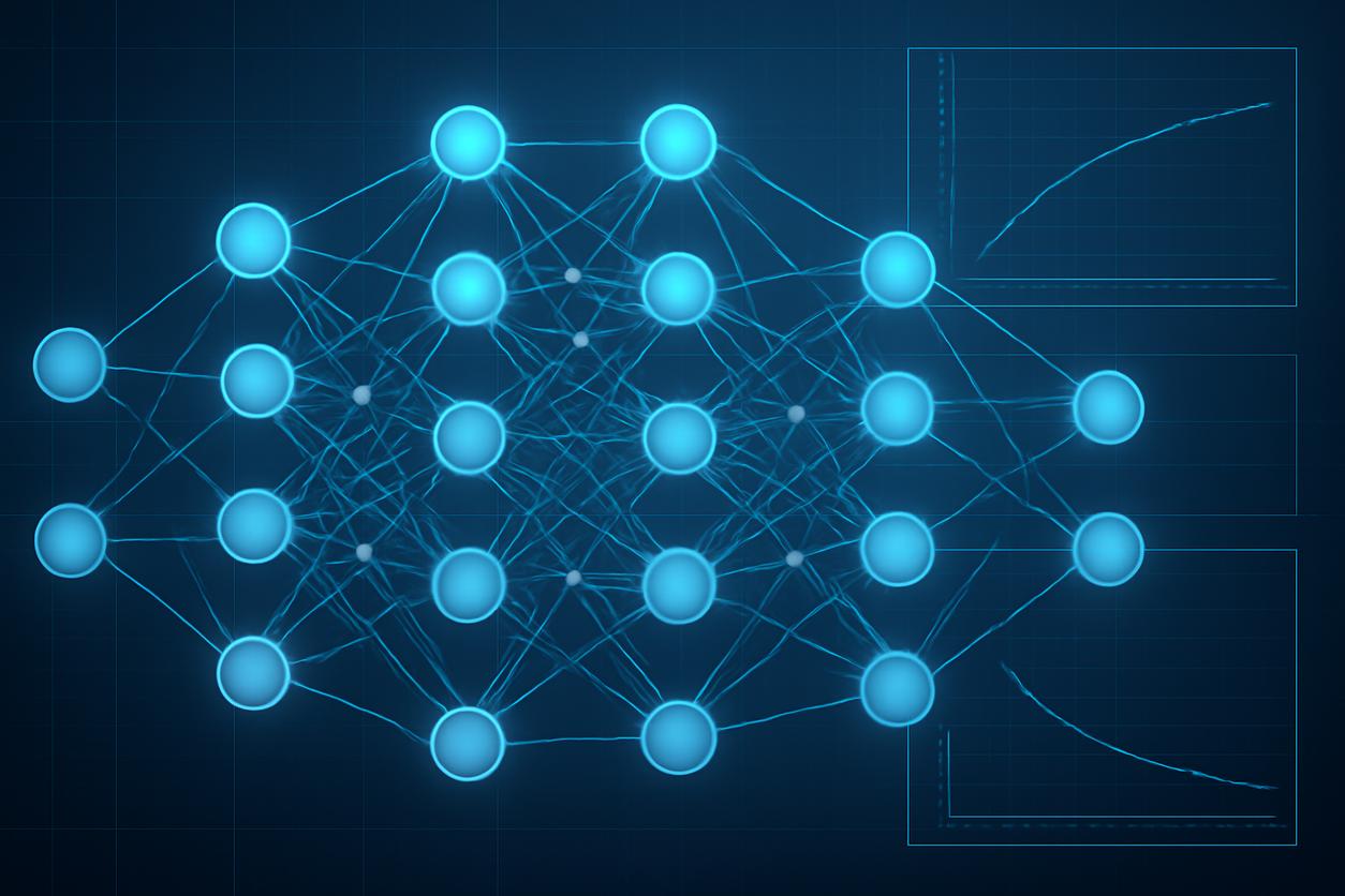
Layers of a Network

A single neuron is limited, but connecting them in layers creates immense power. Most neural networks have at least three types of layers:

• Input Layer: This is the entry point for your data. Each neuron in this layer represents a feature of your dataset (e.g., a pixel in an image or a word in a sentence).
• Hidden Layers: These are the intermediate layers between the input and output. This is where the magic happens. A neural network can have one or many hidden layers, and their job is to detect progressively more complex patterns in the data. The term “deep learning” simply refers to neural networks with many hidden layers.
• Output Layer: This final layer produces the result of the network’s computation, such as a classification (e.g., “cat” or “dog”) or a numerical prediction (e.g., a stock price).

Activation Functions

An activation function is a critical component that introduces non-linearity into the network. Without it, a neural network, no matter how many layers it has, would behave like a simple linear model. Non-linearity allows the network to learn complex relationships between inputs and outputs. Common activation functions include:

• Sigmoid: Squeezes numbers into a range between 0 and 1, often used for binary classification.
• ReLU (Rectified Linear Unit): A popular and efficient choice, it outputs the input directly if it is positive, and zero otherwise.
• Tanh (Hyperbolic Tangent): Similar to sigmoid but squashes values to a range between -1 and 1.

How Learning Happens: Loss, Backpropagation and Optimization

A neural network “learns” by adjusting its weights and biases to make better predictions. This process is an elegant dance between measuring error and systematically correcting it.

Measuring Error: The Loss Function

The first step in learning is to quantify how wrong the network’s predictions are. This is done using a loss function (or cost function). It compares the network’s predicted output to the true, known output and calculates a single number representing the error. For regression tasks, this might be Mean Squared Error (MSE), while for classification, Cross-Entropy Loss is common.

Learning from Mistakes: Backpropagation

Once the error is calculated, the network needs to know how to adjust its internal parameters (weights and biases) to reduce that error. This is the job of backpropagation. Conceptually, backpropagation works backward from the output layer, calculating the contribution of each weight and bias to the total error. It’s like assigning blame for the mistake, layer by layer, allowing the network to make precise adjustments in the right direction.

Finding the Minimum: Optimization Algorithms

Backpropagation tells us the direction to adjust our parameters, but an optimizer determines the size of the step we take. The most fundamental optimizer is Gradient Descent, which iteratively adjusts parameters to find the minimum point of the loss function. More advanced optimizers like Adam and RMSprop adapt the learning rate during training, often leading to faster convergence and better performance.

Architectures Demystified: Feedforward, Convolutional, Recurrent and Transformer Models

Not all neural networks are built the same. Different architectures are designed to solve different types of problems.

Feedforward Neural Networks (FNNs)

This is the simplest type of artificial neural network. Information flows in only one direction—from the input layer, through the hidden layers, to the output layer. FNNs are great for structured data problems, like predicting customer churn or house prices.

Convolutional Neural Networks (CNNs)

CNNs are the masters of spatial data, particularly images. They use specialized layers called convolutional layers that apply filters to an input image, detecting features like edges, corners, and textures. Subsequent layers build on these to recognize more complex objects. They are the technology behind image recognition and object detection systems.

Recurrent Neural Networks (RNNs)

RNNs are designed for sequential data, where order matters, such as time series or text. They have a “memory” loop that allows information to persist from one step in the sequence to the next. This makes them suitable for tasks like language translation and speech recognition. Variants like LSTMs (Long Short-Term Memory) and GRUs (Gated Recurrent Units) solve some of the memory-related challenges of basic RNNs.

Transformer Models

Transformers have revolutionized the field of Natural Language Processing (NLP). Instead of processing data sequentially like RNNs, they use a mechanism called self-attention to weigh the importance of different words in a sentence simultaneously. This allows them to capture complex, long-range dependencies and context, leading to state-of-the-art performance in tasks like text generation and question answering.

Training Strategies: Data, Regularization and Hyperparameter Tuning

Building a great neural network architecture is only half the battle. Effective training is what unlocks its potential.

The Fuel: Data Preparation

Your model is only as good as your data. This involves several steps:

• Cleaning: Handling missing values and removing outliers.
• Normalization/Standardization: Scaling numerical features to a common range (e.g., 0 to 1 or with a mean of 0 and standard deviation of 1) to help the model converge faster.
• Splitting: Dividing the data into training, validation, and test sets to properly evaluate model performance.

Preventing Overfitting: Regularization Techniques

Overfitting occurs when a model learns the training data too well, including its noise, and fails to generalize to new, unseen data. Regularization techniques help prevent this:

• L1 and L2 Regularization: These add a penalty to the loss function based on the size of the model’s weights, discouraging overly complex models.
• Dropout: During training, randomly “drops out” (ignores) a fraction of neurons in a layer. This forces the network to learn more robust features.

Finding the Right Settings: Hyperparameter Tuning

Hyperparameters are the settings you configure before training begins, such as the learning rate, the number of hidden layers, or the dropout rate. Finding the optimal combination is crucial. Looking ahead to 2025 and beyond, training strategies will increasingly leverage automated and sophisticated hyperparameter optimization (HPO) frameworks, moving beyond manual methods like grid search toward more efficient techniques like Bayesian optimization and evolutionary algorithms.

Interpreting Models: Visualization and Explainability Techniques

Deep neural networks are often called “black boxes” because their decision-making processes can be difficult to understand. Model interpretability is the field dedicated to shedding light on how these models work.

Peeking Inside the Black Box

Understanding why a model made a particular prediction is crucial for debugging, building trust, and ensuring fairness. Techniques for Model Interpretability help answer questions like, “Which features were most important for this decision?”

Common Techniques

• SHAP (SHapley Additive exPlanations): A game theory-based approach that explains the prediction of an instance by computing the contribution of each feature.
• LIME (Local Interpretable Model-agnostic Explanations): Explains individual predictions by approximating the complex model locally with a simpler, interpretable one.
• Feature Visualization: Visualizing what individual neurons or layers in a CNN have learned to “see,” such as textures or specific object parts.

Practical Walkthrough: Designing a Simple Classifier Step by Step

Let’s walk through the conceptual steps of building a simple image classifier neural network, such as one that distinguishes between cats and dogs.

1. Define the Problem: The goal is binary classification. Given an image, the model should output a probability that the image contains a cat or a dog.
2. Gather and Preprocess Data: Collect a large dataset of labeled cat and dog images. Resize all images to a standard dimension (e.g., 150×150 pixels) and normalize the pixel values. Split the data into training, validation, and test sets.
3. Choose an Architecture: A Convolutional Neural Network (CNN) is the ideal choice for this task. A simple architecture might consist of a few convolutional and pooling layers followed by a couple of fully connected layers. The final output layer would use a sigmoid activation function to produce a probability between 0 and 1.
4. Train the Model: Choose a loss function (Binary Cross-Entropy), an optimizer (Adam), and a set of hyperparameters. Feed the training data to the model and monitor its performance on the validation set to check for overfitting.
5. Evaluate Performance: Once training is complete, evaluate the final model on the unseen test set to get an unbiased measure of its accuracy and other relevant metrics.

Evaluation and Validation: Metrics and Robust Testing

Accuracy alone can be misleading, especially with imbalanced datasets. A robust evaluation requires a suite of metrics and sound validation techniques.

Beyond Accuracy: Key Metrics

• Precision: Of all the positive predictions, how many were actually correct?
• Recall (Sensitivity): Of all the actual positive cases, how many did the model correctly identify?
• F1-Score: The harmonic mean of precision and recall, providing a single score that balances both.
• AUC-ROC Curve: A plot that illustrates the diagnostic ability of a binary classifier as its discrimination threshold is varied.

Ensuring Generalization: Cross-Validation

K-fold cross-validation is a powerful technique for getting a more reliable estimate of model performance. The data is split into ‘k’ subsets. The model is trained ‘k’ times, each time using a different subset as the test set and the remaining as the training set. The final performance is the average of the ‘k’ runs.

Deployment Notes: From Prototype to Scalable Serving

A trained model is only useful if it can be put into production. Deployment involves transitioning from a research environment to a live system that can serve predictions efficiently and reliably.

Model Optimization

Before deployment, models are often optimized for speed and size without significant loss in accuracy. Techniques include:

• Quantization: Reducing the precision of the model’s weights (e.g., from 32-bit to 8-bit integers).
• Pruning: Removing unnecessary weights or neurons from the network.

Serving Frameworks

Models are typically wrapped in an API (like a REST API) and served using tools like TensorFlow Serving, TorchServe, or custom solutions using containers like Docker. This allows applications to request predictions from the model over a network.

Ethics and Safety: Responsible AI Practices for Models

With great power comes great responsibility. As practitioners, we must be vigilant about the ethical implications of the neural networks we build.

Bias and Fairness

Neural networks learn from data, and if that data contains historical biases (e.g., gender or racial biases), the model will learn and potentially amplify them. Auditing datasets for bias and using fairness-aware machine learning techniques are critical steps in building equitable systems.

Transparency and Accountability

Understanding and documenting how a model works, its limitations, and its intended use case is vital for accountability. This is a key aspect of Responsible AI, ensuring that we can explain and justify the outcomes produced by our models.

Troubleshooting: Common Failure Modes and Remedies

Even experienced practitioners run into issues. Here are some common problems and their potential solutions.

Problem	Potential Cause	Suggested Remedy
Loss is not decreasing	Learning rate is too low or too high; data is not normalized.	Adjust the learning rate; ensure data is properly scaled.
Model is overfitting	Model is too complex; not enough training data.	Add dropout or L2 regularization; use data augmentation.
Model is underfitting	Model is too simple to capture data patterns.	Increase model capacity (more layers or neurons); train for more epochs.
Vanishing/Exploding Gradients	Poor weight initialization; deep network with sigmoid/tanh.	Use ReLU activation; implement batch normalization; use better weight initialization (e.g., He).

Resources for Continued Learning

The journey of learning about neural networks is ongoing. Here are some excellent resources to continue your exploration:

• Deep Learning Book: An in-depth, comprehensive textbook by Ian Goodfellow, Yoshua Bengio, and Aaron Courville. Access it online.
• Reinforcement Learning: Explore a different paradigm of machine learning where agents learn to make decisions by taking actions in an environment. Learn more on Wikipedia.

Summary and Next Steps

We have journeyed from the basic building block of a single neuron to the complex considerations of deploying and monitoring large-scale neural networks. We’ve seen how these models learn through backpropagation, explored the specialized architectures that power modern AI, and touched upon the critical importance of ethics and interpretability. Neural networks are a deep, fascinating, and powerful field. The key to mastery is hands-on practice. Take these concepts, apply them to a project you are passionate about, and continue to build on this foundational knowledge.