Practical Reinforcement Learning: Concepts and First Experiments

A Practical Guide to Reinforcement Learning: From Core Concepts to Implementation

Table of Contents

• Overview: Why Reinforcement Learning Matters
• Core Concepts: Agents, States, Rewards, and Policies
• Mathematical Foundation: Markov Decision Processes
• Model-Free Approaches: Value-Based Learning and Policy Optimization
• Model-Based Techniques and Planning Strategies
• Exploration Methods and Improving Sample Efficiency
• Practical Lab: Building a Simple Agent with Pseudocode
• Evaluation: Metrics, Debugging, and Stability Checks
• Ethics, Safety, and Responsible Use in Deployments
• Further Reading and Reproducible Resources

Overview: Why Reinforcement Learning Matters

In the vast landscape of machine learning, three paradigms stand out: supervised learning, unsupervised learning, and the uniquely powerful field of Reinforcement Learning. While supervised learning learns from labeled data and unsupervised learning finds patterns in unlabeled data, Reinforcement Learning (RL) learns through interaction. It is the science of making optimal decisions based on trial and error, much like how a pet learns a new trick by receiving treats for good behavior.

This interactive learning process is what makes Reinforcement Learning so compelling. It allows us to train agents to master complex, sequential decision-making tasks in dynamic environments, from playing sophisticated games like Go and StarCraft to controlling robotic arms, optimizing chemical reactions, and managing financial portfolios. For intermediate practitioners, understanding RL opens a new frontier of problems that cannot be solved with static datasets alone. This guide provides an intuition-first, framework-agnostic path to mastering the core principles of this exciting domain.

Core Concepts: Agents, States, Rewards, and Policies

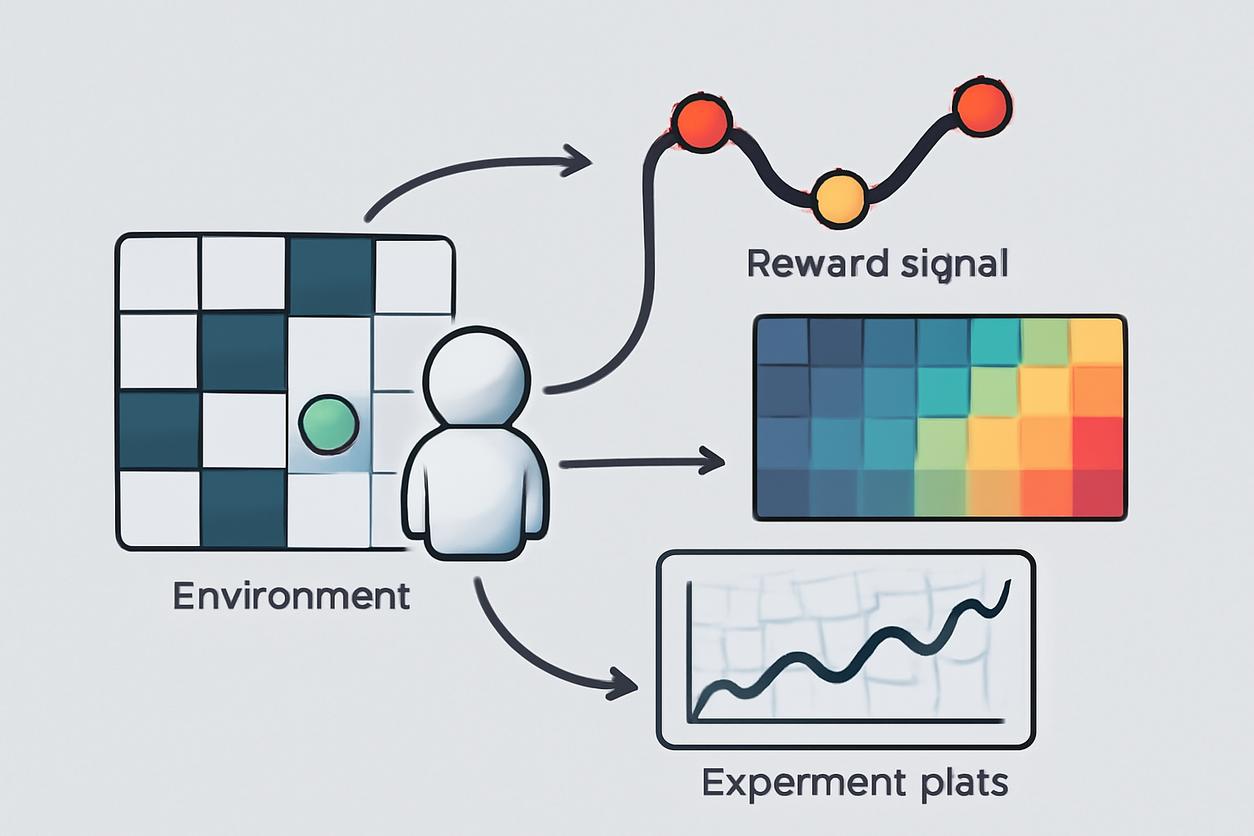
To grasp Reinforcement Learning, we must first understand its fundamental vocabulary. Imagine training a mouse (our agent) to navigate a maze (the environment) to find a piece of cheese (the reward). This simple analogy helps illustrate the key components.

The Core Loop

The entire process operates in a continuous loop:

1. The agent observes the current state of the environment.
2. Based on this state, the agent chooses an action according to its policy.
3. The environment responds by transitioning to a new state and providing a reward signal.
4. The agent uses this reward to update its policy, improving its decision-making for the future.

Key Components Explained

• Agent: The learner or decision-maker. In our analogy, the mouse. In a real-world application, this could be the algorithm controlling a robot or a trading bot.
• Environment: The world in which the agent operates. For the mouse, it’s the maze. The environment defines the rules, the states, and how actions affect those states.
• State (S): A snapshot of the environment at a specific moment. This is the information the agent uses to make a decision. A state could be the mouse’s coordinates (x, y) in the maze.
• Action (A): A move the agent can make. The mouse’s possible actions are moving up, down, left, or right.
• Reward (R): The feedback signal from the environment. It tells the agent how good or bad its last action was. Finding cheese yields a positive reward (+10), stepping on a trap yields a negative reward (-5), and an uneventful move yields a neutral or small negative reward (0 or -0.1 to encourage speed). The agent’s goal is to maximize the cumulative reward over time.
• Policy (π): The agent’s strategy or “brain.” It maps states to actions. A simple policy might be, “If you see a wall to your right, turn left.” A complex policy, learned through training, is a sophisticated function that determines the best action to take in any given state to maximize future rewards.

Mathematical Foundation: Markov Decision Processes

While the mouse-in-a-maze analogy provides intuition, the formal framework for Reinforcement Learning problems is the Markov Decision Process (MDP). An MDP is a mathematical model for sequential decision-making where outcomes are partly random and partly under the control of a decision-maker. It assumes the Markov property: the future is independent of the past, given the present. In other words, the current state provides all the necessary information to make an optimal decision.

The MDP Tuple

An MDP is defined by a set of components, often represented as a tuple (S, A, P, R, γ):

• S: A finite set of all possible states.
• A: A finite set of all possible actions.
• P: The transition probability function, P(s’ | s, a). This defines the probability of transitioning to state s’ after taking action a in state s. It represents the environment’s dynamics. For example, if a robot tries to move forward, there might be a 90% chance it succeeds and a 10% chance its wheels slip and it stays in the same place.
• R: The reward function, R(s, a, s’). This defines the immediate reward received after transitioning from state s to s’ by taking action a.
• γ (Gamma): The discount factor, a value between 0 and 1. It determines the importance of future rewards. A gamma of 0 makes the agent completely myopic (only caring about immediate rewards), while a gamma close to 1 makes it far-sighted, valuing long-term gains. This prevents infinite returns in cyclical problems and reflects the general preference for immediate rewards over distant ones.

The goal of a Reinforcement Learning agent in an MDP is to find a policy π that maximizes the discounted cumulative reward, also known as the return.

Model-Free Approaches: Value-Based Learning and Policy Optimization

Model-free methods are the workhorses of modern Reinforcement Learning. They learn a policy directly from experience without building an explicit model of the environment’s dynamics (the P and R functions). This is useful when the environment is too complex to model, which is often the case in the real world. There are two main families of model-free algorithms.

Value-Based Learning

Value-based methods learn a value function that estimates the expected return from being in a particular state or taking a specific action. The policy is then derived implicitly by choosing the action that leads to the highest value.

• Q-Learning: A classic and highly influential value-based algorithm. It learns an action-value function, Q(s, a), which represents the expected return of taking action a in state s and then following an optimal policy thereafter. The Q-values are updated iteratively using the Bellman equation, which relates the value of the current state-action pair to the value of the next. The agent’s policy is to simply choose the action with the highest Q-value in the current state (this is a greedy policy). For more details, see the Q-learning entry.

Policy Optimization

Instead of learning a value function, policy optimization methods learn the policy π directly. The policy is represented as a parameterized function (e.g., a neural network) that outputs a probability distribution over actions for a given state.

• Policy Gradient Methods: These algorithms adjust the policy’s parameters by performing gradient ascent on the expected return. The core idea is simple: if taking an action in a certain state led to a high reward, increase the probability of taking that action in that state in the future. Conversely, if it led to a low reward, decrease its probability. This approach is particularly effective in continuous action spaces and for learning stochastic policies. Popular examples include REINFORCE and Actor-Critic methods. You can learn more about policy gradient methods here.

Model-Based Techniques and Planning Strategies

In contrast to model-free approaches, model-based Reinforcement Learning algorithms attempt to learn a model of the environment. This model is essentially an approximation of the transition function P and the reward function R. Once the agent has this internal model, it can use it to “simulate” future outcomes and plan ahead without having to interact with the real environment.

The Advantage of a Model

The primary benefit of model-based RL is sample efficiency. Real-world interactions can be expensive or slow (e.g., in robotics). By learning a model, the agent can generate a large amount of simulated experience and use it for planning, drastically reducing the number of real-world samples needed. Algorithms like Dyna-Q interleave real interactions, model learning, and simulated planning to accelerate the learning process.

Planning with a Model

Once a model is learned, the agent can use planning algorithms like value iteration or tree search (e.g., Monte Carlo Tree Search) to find an optimal policy within its simulated world before ever taking another real step.

Exploration Methods and Improving Sample Efficiency

A fundamental challenge in Reinforcement Learning is the exploration-exploitation tradeoff. The agent must exploit its current knowledge to maximize rewards, but it must also explore the environment to discover potentially better actions and states it hasn’t encountered yet. An agent that only exploits might get stuck in a suboptimal routine, while an agent that only explores will never capitalize on its discoveries.

Classic and Modern Strategies

• Epsilon-Greedy: A simple yet effective strategy. With probability ε (epsilon), the agent chooses a random action (explore). With probability 1-ε, it chooses the action with the highest estimated value (exploit). Typically, ε starts high and is gradually decreased over time.
• Upper Confidence Bound (UCB): This method encourages exploration of actions with high uncertainty. It selects actions based on both their estimated value and an “uncertainty bonus.” Actions that haven’t been tried often will have high uncertainty and are thus more likely to be chosen.
• Future Strategies for 2025 and Beyond: As we look to advanced strategies in 2025 and onward, the focus is shifting toward more intelligent exploration. Techniques based on intrinsic motivation will become more refined. Instead of relying on random chance, agents will be driven by curiosity, seeking out novel or surprising states. These curiosity-driven agents build a model of their world and are rewarded for visiting states that their model predicts poorly, effectively pushing them to explore the most informative parts of the environment.

Practical Lab: Building a Simple Agent with Pseudocode

Let’s solidify these concepts with a simple grid-world problem. The agent (A) must navigate a 4×4 grid to reach the Goal (G) while avoiding the Pit (P). The Start (S) is at (0,0).

Environment:

• States: 16 grid positions (0-15).
• Actions: Up, Down, Left, Right.
• Rewards: +10 for reaching G, -10 for falling into P, -0.1 for any other move (to encourage efficiency).

Q-Learning Pseudocode

We will use Q-learning to solve this. The agent will maintain a Q-table, a lookup table storing the Q-value for each state-action pair.

Initialize Q-table with all zeros: Q[16 states][4 actions] = 0Set learning rate (alpha) = 0.1Set discount factor (gamma) = 0.9Set exploration rate (epsilon) = 1.0Set max epsilon = 1.0, min epsilon = 0.01, decay rate = 0.001FOR episode in 1 to total_episodes:    Initialize state = Start State (0)    Initialize done = false    WHILE not done:        // Exploration-exploitation trade-off        IF random_number 

After training, the Q-table will contain the optimal action-values, and the agent can find the goal by always choosing the action with the highest Q-value from its current state.

Evaluation: Metrics, Debugging, and Stability Checks

Evaluating a Reinforcement Learning agent is not as straightforward as measuring accuracy on a test set. Since the agent learns online, its performance must be tracked over time.

Key Evaluation Metrics

• Cumulative Reward per Episode: This is the most fundamental metric. A good agent should show a clear upward trend in the total reward it accumulates in each episode as training progresses.
• Episode Length: For goal-oriented tasks, a shorter episode length often indicates a more efficient policy.
• Time to Convergence: How many episodes or time steps does it take for the agent's performance to plateau?

Common Debugging Challenges

Reinforcement Learning is notoriously difficult to debug. Common pitfalls include:

• Hyperparameter Sensitivity: The learning rate, discount factor, and exploration parameters can drastically affect performance. Grid search or more advanced hyperparameter optimization techniques are often necessary.
• Reward Shaping: A poorly designed reward function can lead to unintended behaviors (reward hacking). The rewards must precisely specify the desired outcome.
• Instability: In deep RL, training can be unstable. Plotting the loss function and reward curves is essential to diagnose issues like divergence or catastrophic forgetting.

Ethics, Safety, and Responsible Use in Deployments

As Reinforcement Learning systems move from simulations to the real world, considering their ethical implications and safety is paramount. An agent optimized to maximize a specific reward signal may discover harmful or undesirable ways to achieve its goal.

Key Considerations

• Reward Hacking: An agent might find a loophole in the reward function. For example, a cleaning robot rewarded for the amount of dirt collected might learn to dump its dustbin and re-collect the same dirt to maximize its reward.
• Unintended Side Effects: An agent may alter the environment in negative ways that were not part of its reward function. For instance, a robot trying to move a box might scratch the floor in the process.
• Safe Exploration: In physical systems like robotics or self-driving cars, purely random exploration can be dangerous. The agent must be constrained to explore only safe actions during its learning phase.

Developing responsible Reinforcement Learning requires careful reward design, robust safety constraints, and continuous human oversight, especially in high-stakes applications.

Further Reading and Reproducible Resources

This guide has provided a foundational overview of Reinforcement Learning. To deepen your understanding, we highly recommend the following resources:

• The Foundational Textbook: Reinforcement Learning: An Introduction by Sutton and Barto is the definitive text in the field.
• A Comprehensive Survey: For an overview of modern techniques, especially those combined with deep learning, this Survey of Deep Reinforcement Learning is an excellent resource.

By combining a strong grasp of the core concepts with hands-on practice and a commitment to responsible implementation, you can unlock the immense potential of Reinforcement Learning to solve some of the most challenging problems in AI today.