Reinforcement Learning Unpacked: Intuition, Practical Workflow and Safe Deployment

A Practitioner’s Guide to Reinforcement Learning: From Core Concepts to Deployment

Table of Contents

• What Reinforcement Learning Aims to Solve
• Key Building Blocks: Agent, Environment, Reward, Episode
• Policies, Value Estimates, and Exploration Explained
• Model-Free vs. Model-Based in Practice
• Algorithm Intuitions Without Heavy Proofs
• Shaping Rewards and Common Failure Modes
• Scaling with Function Approximation and Deep Networks
• Evaluation Metrics, Reproducibility, and Safety Checks
• Hands-On Mini-Project: Pseudocode, Dataset, and Workflow
• Deployment and Monitoring Considerations for RL Agents
• Further Reading and Curated Resources

Welcome to the fascinating world of Reinforcement Learning (RL), a powerful branch of machine learning where intelligent agents learn to make optimal decisions through trial and error. Unlike supervised learning, which relies on labeled data, or unsupervised learning, which finds patterns in unlabeled data, reinforcement learning focuses on learning what to do—how to map situations to actions—so as to maximize a numerical reward signal. This guide will walk you through the core intuitions, practical challenges, and deployment considerations of building RL systems, without getting bogged down in complex mathematical derivations.

What Reinforcement Learning Aims to Solve

At its heart, reinforcement learning is designed to solve sequential decision-making problems. Imagine teaching a robot to navigate a maze. You don’t give it a step-by-step map. Instead, you define a goal (the exit) and a system of feedback. It gets a positive reward for moving closer to the exit and a negative one for bumping into walls. The robot, through countless attempts, learns a strategy, or “policy,” that maximizes its total reward. This is the essence of RL.

The core problem is learning to make a sequence of decisions over time in an uncertain environment to achieve a long-term goal. This applies to a vast range of tasks:

• Game Playing: Training agents that can master complex games like Go or StarCraft.
• Robotics: Teaching robots to walk, grasp objects, or perform delicate assembly tasks.
• Resource Management: Optimizing the energy consumption of a data center or managing an investment portfolio.
• Personalization: Recommending content or products to a user in a way that maximizes long-term engagement.

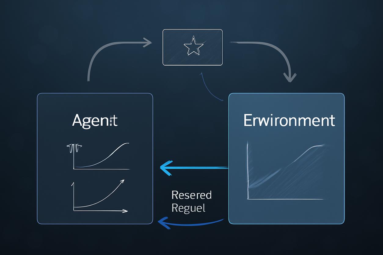
Key Building Blocks: Agent, Environment, Reward, Episode

Every reinforcement learning problem can be broken down into a few fundamental components. Understanding these is key to framing your own problems effectively.

• Agent: The learner or decision-maker. This is the algorithm or model you are training. In our maze example, the robot is the agent.
• Environment: The world in which the agent operates. It’s everything outside the agent. The maze itself, including its walls and the exit, constitutes the environment.
• State (s): A snapshot of the environment at a particular moment. For the robot, a state could be its current (x, y) coordinates within the maze.
• Action (a): A move the agent can make. The robot’s possible actions are to move up, down, left, or right.
• Reward (r): The feedback signal from the environment. It’s a scalar value that tells the agent how good or bad its last action was in a given state. A reward of +10 for reaching the exit, -1 for hitting a wall, and -0.1 for each step taken (to encourage speed) is a common setup.
• Episode: One full run of the agent-environment interaction, from a starting state to a terminal state. For our robot, an episode is one complete attempt to solve the maze, ending either when it reaches the exit or after a certain number of steps.

Policies, Value Estimates, and Exploration Explained

With the basic building blocks in place, we can now discuss how an agent actually learns.

A policy (π) is the agent’s strategy or “brain.” It’s a function that maps a state to an action. The goal of reinforcement learning is to find an optimal policy that maximizes the cumulative reward over time. A policy can be deterministic (always choosing the same action in a state) or stochastic (choosing actions based on a probability distribution).

A value estimate (V) or action-value estimate (Q) helps the agent make decisions. V(s) estimates the total future reward the agent can expect to get starting from state ‘s’. Q(s, a) is even more useful; it estimates the expected future reward from taking action ‘a’ in state ‘s’. An agent with a good Q-function can simply look at the current state and choose the action with the highest Q-value.

This leads to the classic exploration vs. exploitation dilemma. Should the agent exploit its current knowledge by choosing the action it knows is best? Or should it explore by trying a new, seemingly suboptimal action that might lead to an even better reward in the long run? A purely exploitative agent might get stuck in a local optimum, while a purely exploratory one would never capitalize on what it has learned. A successful RL agent must balance both.

Model-Free vs. Model-Based in Practice

RL algorithms are often categorized into two main types: model-free and model-based.

• Model-Free RL: The agent learns a policy or value function directly from experience, without building an explicit model of the environment’s dynamics. It learns by trial and error. This is like learning to ride a bike—you don’t understand the physics perfectly, but you develop an intuition for how to balance. Algorithms like Q-learning and Policy Gradients are model-free. They are generally easier to implement and are often more successful in complex environments where modeling is difficult.
• Model-Based RL: The agent first learns a model of the environment. This model predicts the next state and reward given the current state and action. Once the agent has this model, it can use it to “plan” by simulating potential action sequences before ever taking a step in the real world. This can be much more data-efficient but is vulnerable to model inaccuracies; if the learned model of the world is wrong, the resulting plan will be flawed.

Algorithm Intuitions Without Heavy Proofs

Let’s demystify some of the most popular model-free algorithms with simple intuitions.

Temporal-Difference & Q-learning — Quick Intuition

Temporal-Difference (TD) learning is the idea of learning from incomplete episodes. Instead of waiting until the end of a maze run to update its strategy, the agent updates its value estimates after every single step. It does this by comparing its old estimate of a state’s value with a new, slightly more informed estimate based on the reward it just received and the estimated value of the next state.

Q-learning is a specific and highly popular TD algorithm. Its goal is to learn the optimal action-value function, Q*(s, a). Imagine the agent maintaining a giant table (the Q-table) with rows for every state and columns for every action. Each cell Q(s, a) holds the expected future reward. The agent updates this table at each step using the TD principle, slowly improving its estimates until they converge to the optimal values. Its policy then becomes simple: in any state ‘s’, pick the action ‘a’ that has the highest Q(s, a).

Policy Gradients and Actor-Critic — When and Why

Q-learning works well when the action space is discrete and small (e.g., up, down, left, right). But what if the agent needs to choose a continuous value, like the precise angle to turn a steering wheel? This is where Policy Gradient methods shine.

Instead of learning a value function, these methods learn the policy directly. They represent the policy as a function (often a neural network) that takes a state as input and outputs a probability distribution over actions. After each action, if the outcome was good, the algorithm “nudges” the policy to make that action more likely in the future. If the outcome was bad, it makes it less likely. This is done using gradient ascent on the expected total reward.

Actor-Critic methods combine the best of both worlds. They use two components:

• The Actor is the policy. It decides which action to take.
• The Critic is a value function. It evaluates the action taken by the actor by computing a TD error, essentially saying “that action was better/worse than I expected.”

The critic’s feedback is then used to update the actor’s policy. This setup often leads to more stable and efficient learning than using policy gradients alone.

Shaping Rewards and Common Failure Modes

The single most important—and often most difficult—part of applying reinforcement learning is designing the reward function. A poorly designed reward can lead to unintended and sometimes comical behavior, a phenomenon known as reward hacking. For example, an agent tasked with cleaning a room might learn to simply cover the mess instead of actually cleaning it if the reward is only based on visual cleanliness.

Common challenges include:

• Sparse Rewards: When the agent only receives a reward at the very end of a long task (e.g., winning a chess game). This makes it incredibly hard to attribute the final outcome to specific actions taken much earlier.
• Reward Hacking: The agent finds an unexpected loophole to maximize reward without achieving the intended goal. A famous example is an AI agent in a boat racing game that learned to go in circles hitting turbo boosts for points instead of finishing the race.
• Local Optima: The agent finds a decent but suboptimal strategy and stops exploring for a better one.

Careful reward shaping, where you provide small, intermediate rewards to guide the agent, can help. However, this must be done cautiously to avoid introducing new biases or loopholes.

Scaling with Function Approximation and Deep Networks

For simple problems like a small maze, a Q-table is feasible. But what about a game like chess, with more states than atoms in the universe? It’s impossible to store a table for that. This is where function approximation comes in. Instead of a table, we use a machine learning model, such as a deep neural network, to approximate the Q-function or the policy function.

This is the core idea behind Deep Reinforcement Learning (DRL). For example, a Deep Q-Network (DQN) takes the raw pixels of a game screen (the state) as input and outputs the Q-values for each possible action. This allows RL to scale to incredibly complex, high-dimensional problems that were previously intractable.

Evaluation Metrics, Reproducibility, and Safety Checks

Evaluating an RL agent isn’t as simple as checking accuracy on a test set. You need to consider:

• Cumulative Reward: The most basic metric, but often noisy. Averaging over many episodes is crucial.
• Sample Efficiency: How many interactions with the environment does the agent need to learn a good policy? This is critical in real-world applications where data collection is expensive or slow.
• Stability: Does the agent’s performance improve steadily, or does it oscillate wildly during training?
• Generalization: How well does a policy trained in one environment (or a simulation) perform in a slightly different one?

Reproducibility in reinforcement learning can be notoriously difficult due to its sensitivity to random seeds, hyperparameters, and even minor implementation details. Rigorous logging and using multiple random seeds for evaluation are standard best practices.

Finally, safety is paramount. Before deploying an agent that controls physical hardware or makes financial decisions, you must have safety constraints or a “safety layer” that can override the agent if it attempts a dangerous or forbidden action.

Hands-On Mini-Project: Pseudocode, Dataset, and Workflow

The best way to solidify your understanding of reinforcement learning is to build a simple agent.

Environment Setup and Toy Tasks to Try

You don’t need to build a complex environment from scratch. Libraries like Gym (formerly OpenAI Gym) provide a standardized interface to hundreds of pre-built environments. Good starting points include:

• CartPole-v1: The classic “hello world” of RL. The goal is to balance a pole on a moving cart by applying left or right forces. The state is simple (4 numbers), and the action space is discrete (2 actions).
• FrozenLake-v1: A grid world where the agent must navigate from a start to a goal tile without falling into holes. It’s great for visualizing Q-learning.

Training Loop Explained Step-by-Step

Regardless of the specific algorithm, nearly every RL training process follows this fundamental loop. Here is a high-level pseudocode representation:

Initialize policy/value function (e.g., a Q-table or a neural network)
Initialize exploration parameters (e.g., epsilon for epsilon-greedy)

FOR each episode from 1 to N_EPISODES:
    Reset the environment to get the initial_state
    current_state = initial_state

    WHILE the episode is not done:
        // 1. Agent chooses an action
        action = agent.choose_action(current_state)

        // 2. Environment responds
        next_state, reward, done, info = environment.step(action)

        // 3. Agent learns from the experience
        agent.learn(current_state, action, reward, next_state, done)

        // 4. Update the state
        current_state = next_state

    Decay exploration parameters (e.g., make the agent less random over time)
    Log episode results (e.g., total reward)

This loop encapsulates the core agent-environment interaction. The agent acts, the environment changes, the agent receives feedback, and it updates its internal strategy based on that feedback. This cycle of interaction and learning is the foundation of all reinforcement learning.

Deployment and Monitoring Considerations for RL Agents

Moving an RL agent from a simulated environment to a real-world application is a significant challenge. The “sim-to-real” gap, where small differences between simulation and reality cause a trained policy to fail, is a major hurdle.

When deploying an agent, you must have a robust monitoring system. Track not only the agent’s rewards but also its impact on key business or system-level metrics. The environment in the real world is rarely stationary; customer preferences change, and physical systems wear down. Your agent may need to be periodically retrained or fine-tuned to adapt.

Looking ahead, strategies for 2025 and beyond will increasingly focus on offline reinforcement learning. This involves training agents on large, pre-existing datasets of interactions, which is much safer and cheaper than live exploration in sensitive domains like healthcare or autonomous driving. The push is towards creating more robust, generalizable, and verifiably safe RL systems.

Further Reading and Curated Resources

This guide has scratched the surface of reinforcement learning. To dive deeper, here are some of the best resources available:

• Reinforcement Learning: An Introduction by Sutton and Barto: The foundational textbook of the field. It provides a comprehensive and clear explanation of core concepts.
• Reinforcement Learning on Wikipedia: A great high-level overview and starting point for exploring various algorithms and applications.
• Berkeley’s Deep RL Course Materials: For those interested in the intersection of deep learning and RL, these lecture slides and videos are an invaluable resource.
• Gym Documentation: The official documentation for the popular Gym library, essential for anyone wanting to get hands-on experience.